On December 15th, I had the pleasure of presenting a session of “Introduction to Deep Learning” at the recently held #globalAIBootcamp (an amazing event with 68 participating locations worldwide).

This blog post captures some of the key points from my presentation. Feel free to go directly to the slides located here.

Before I begin, I would like to thank François Chollet for his excellent book “Deep Learning with Python.” In my almost four-year quest to better understand deep learning, I found his book to be one of the best written books on this topic.

(I will totally understand if, at this point, you abandon reading this blog post and start reading François Chollet’s book…in fact, I recommend you do just that 😊)

The Importance of Deep Learning for Developers

Deep learning is such an incredible tool for developers like us. Deep learning has already helped solve complex problems such as near-human level image classification, handwriting recognition, speech recognition and more. Much of this aforementioned functionality is now available to us in the form of an easily callable API (e.g. Cognitive Services). Furthermore, many of these APIs also allow us to train the underlying models using data from our own specific domains (e.g. Custom Speech API). Finally, with the advent of automated ML tools, there is now a WYSIWYG way to get started with deep learning (e.g. Lobe.AI).

If we have all these tools available, why would we, as developers, need to code deep learning models from scratch?

To answer this question, let us review a recent quote from Andrew Ng.

“AI (Artificial Intelligence) technology is now poised to transform every industry, just as electricity did 100 years ago. Between now and 2030, it will create an estimated $13 trillion of GDP growth. While it has already created tremendous value in leading technology companies such as Google, Baidu, Microsoft and Facebook, much of the additional waves of value creation will go beyond the software sector.”

In addition to the astounding number in itself, the important part of this quote is the bold text (emphasis is mine). Large software companies have already created tremendous value for themselves through speech recognition, object classification, language translation, etc., and now it is up to us as developers to take this technology to our customers beyond the software sector. Bringing deep learning solutions to these sectors may, in many cases (but not all), require developing our own custom deep learning models. Here are a few examples:

1. Predicting patient health outcomes based on past health data
2. Mapping a set of attributes about a product to predict manufacturing defects
3. Mapping pictures of food items to prices and calorie count for a self-checkout kiosk
4. Smart bots for a specific industry
5. Summarization of a vast amount of text into an auto-generated short summary with a timeline

In order to develop these kinds of solutions, I believe that we need to have a working knowledge of deep learning and neural networks (also referred to as Artificial Neural Networks or ANNs).

What is Deep Learning?

But what is a neural network and what do I mean by “deep” in deep learning? A neural network is a layered structure that is “inspired” by the neurons in our brain.

Like the neurons in our brain, which are essentially a network of cells that get activated or inhibited (think 0 or 1) based on an incoming signal, a neural network is comprised of layers of cells that are activated or inhibited by an incoming signal. As we will see later, in the case of a neural network, the cells can store any value (instead of just binary values).

Despite the similarities, it is unclear whether neurons in our brain work in a similar way to the neurons in neural networks. Thus, I emphasized the word “inspired” earlier in this paragraph. Of course, that has not stopped the popular press from painting a magical picture around deep learning (now you know not to buy into this hype).

We still need to answer our question about the meaning of the word “deep” in deep learning. As it turns out, a typical neural network is multiple levels deep – hence the reference to “deep” in deep learning. It’s that simple!

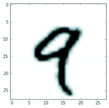
Let us change gears and look briefly into what we mean by “learning.” We will use the “Hello World” equivalent for neural nets as the basis for our explanation. This is a neural network that can identify a handwritten digit (such as the one shown below).

It’s All About a Layered Network

Input Layer

Let’s think of a neural network as a giant data transformation engine that takes a handwritten image as input and outputs a number between 0-9. Under the cover, a handwritten image is really a matrix of, say, 28 X 28 cells, with each cell’s value ranging from 0-255. A value of 0 represents white and a value of 255 represents black. So altogether we have 28 X 28 (784) cells in the input layer.

Hidden Layer

Now let us, somewhat arbitrarily, add a layer underneath the input layer (because this layer is underneath the input layer, it is referred to as a “hidden” layer). Furthermore, let us assume that we have 512 cells in the hidden layer (compared to 784 cells in the input layer). Now imagine that each cell in the input layer is connected to each cell in the hidden layer – this is referred to as densely connected layers.

Each connection, in turn, has a multiplier (referred to as a weight) associated with it that drives the value of the cell in the next layer as shown. To help visualize this, please refer to the diagram below: The lines in red show all the incoming connections coming into the topmost cell of the hidden layer. The numbers decorating the incoming connections are the associated weights that drive the value of cells in the hidden layer.

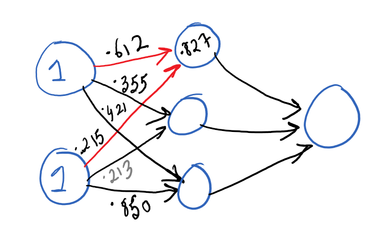
For example, the topmost cell in the hidden layer gets a value of .827 – we got this value by adding the weight of each input cell and multiplying it by a weight (i.e. 1 * .612 + 1 * .215). Stated differently, we have calculated the value of the cell in the hidden layer using the weighted sum of all the incoming connections.

Weighted Sum, Bias and Activation Function

The weighted sum calculation is rather simplistic. We want this calculation to be a bit more sophisticated, so we can conduct more complex transformations as the data flows from one layer to next (after all, we are trying to teach our network the non-trivial problem of identifying handwritten digits).

In order to make the weighted sum calculation a bit more sophisticated, we can do a couple of things to help us control how data flows to the following layer:

1. We can introduce a notion of threshold associated with the weighted sum – if the weighted sum is below a certain threshold, we will consider the next neuron not to be activated. An easy way to incorporate the notion of the threshold in our weighted sum calculation is to add an equivalent constant value to it (referred to as a bias).
2. We introduce the notion of an activation function. Activation functions are mathematical functions like Sigmoid and ReLU that can transform the output of the neuron. For example, ReLU is simply a max operation that returns a value of 0 if the input value is a negative number; else it simply returns the input value. Here is the C# code snippet to implement ReLU:

public double calcReLU (double x){return Math.Max(0,x);}

If you are wondering why the weighted sum calculation is simplistic and why we needed to add things like a bias and activation function, it is helpful to note that, ultimately, ML boils down to searching for the right data transformation function (consistent with our earlier statement that at the highest level, ML is really about transforming input data into output data).

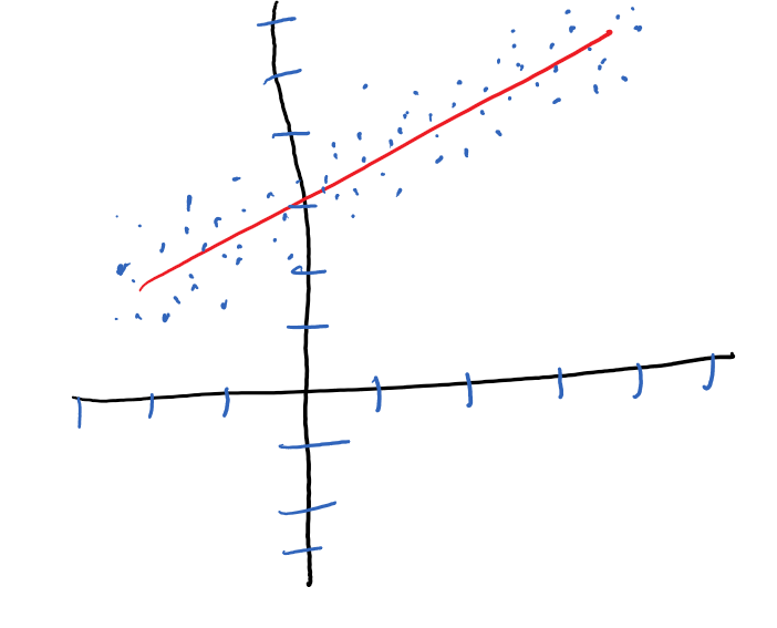
For example, in the diagram below, our ML program has “learnt” to predict a value of y, given x, using the training set. The training set is made of a collection of (x,y) coordinates depicted as blue dots. The “learnt” data transformation (depicted as the red line in the diagram) is a simple linear data transformation.

If the data transformation that the ML routine was supposed to learn was more complex than the example above, we will need to widen our search space (also referred to a hypothesis space). This is when introducing the concepts like bias and activation function can help. In the diagram below, the ML program needs to learn a more complex data transformation logic.

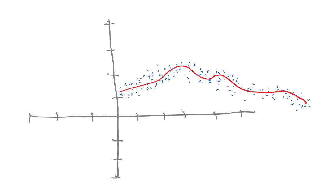
You are probably wondering how ReLU can help here – after all, the ReLU / max operation seems like another linear transformation. This is not true: ReLU is a non-linear transformation function. In fact, you can chain multiple ReLU operations to mimic a non-linear graph, such as the one shown in the diagram above.

Recognizing  Patterns

Before we leave this section, let us ponder for a moment about the weighted sum calculation and activation function. Based on what we have discussed so far, you understand that the weighted sum and the activation function together help us calculate the value of the cell in the next layer. But how does a calculation such as this help the neural net recognize handwritten digits?

The only way a neural network can learn to recognize digits is by finding patterns in the image, i.e., the number “9” is a combination of a circle alongside a vertical line. If we had to write a program to detect a vertical line in the center of an image, what would we do? We have already talked about representing an image as a 28 X 28 matrix, where each cell of the matrix has a value of 0-255. One easy way to determine if this image has a vertical line in the center of the image is to create another 28 X 28 matrix and set high values for cells where we are looking for the vertical line and low values for cells everywhere else.

Now if we multiply the two matrices, assuming our image did indeed have a vertical line in the center of the image, we will end up with a matrix that will have high values for cells that make up the vertical line. Hopefully, you have begun to develop an intuition on how the neural network will learn to recognize handwritten digits. (Note – on its own, we are not providing it a cheat sheet of patterns for each digit.)

Output Layer

Finally, let’s add an output layer that has only 10 cells. Why just 10 cells? Remember that the purpose of a neural net is to predict the digit that corresponds to a handwritten digit. This means we have 10 possibilities (0-9). Each cell of our output layer will contain a probability score of what our neural network thinks is the handwritten digit (the sum of all the probabilities cannot exceed 1). Such an output layer is referred to as a SoftMax layer.

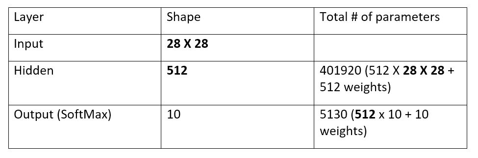
With the necessary layers in place, let us review the layers in our neural network model as shown in the table below. The input layer is a 28 X 28 matrix of pixels. The hidden layer is comprised of 512 cells and the output layer has 10 cells. The third column of the table depicts the total number of weight parameters that can be adjusted for the network to learn.

What is “Learning”?

Great! We now have a neural network in place! But why is it even reasonable to think that a layered structure can learn to recognize handwritten digits?

This is where learning comes in!

We will start out by initializing the weights to some random values. Then we will go about calculating the values of cells in the hidden layer, and subsequently, the values in the output layer – this process is referred to as a forward pass. Since we initialized the weights to random values, we cannot expect the output to be a meaningful value.

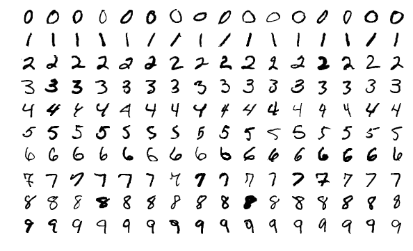
Of course, our predicted output is going to be wrong. But how wrong? Well… we can calculate the difference between our incorrect output and “correct” output. I suspect that you’ve heard that in order to conduct the learning, we need a set of training examples – in our case, images of handwritten digits and the “correct” answer (referred to as “labels”). Fortunately for us, folks behind the MNIST database have already created a training set that is comprised of images of 60,000 handwritten digits and the corresponding labels. Here is an image depicting sample images from the MNIST database.

Note: When working on a real-world problem, you probably won’t find a readily available training set. As you can imagine, collecting the requisite sized training set is one of the key challenges you will face. More training data is almost always better when it comes to neural network learning. (Although, there are techniques like data augmentation that can allow you to get by using a smaller training set.)

Another real-world challenge is the required data wrangling to transform the data into a format that is conducive for feeding into a neural network. The process of using knowledge of your context to transform the data into a format that makes neural network learning work better is known as feature engineering. One of the strengths of neural networks is that it can conduct its own feature discovery by itself (unlike other forms of machine learning). We don’t have to tell the neural network that the digit 9 is made up of a circle and a vertical line.

That said, any data transformation you can undertake in order to ease the learning will lead to a more optimal solution (in terms of resource and training set requirements).

Since we know the correct answer to our “identify the handwritten digit” question, we can determine how wrong we were with the output. But rather than using the simple difference between the two, let us be a bit more mathematically sound and use the square of the differences between the incorrect and correct output values. This way we take into account negative values. This calculation (the squared difference) is referred to as a loss function.

A related concept is cost – it represents the sum of all the loss values added up over the entire training set – in this case, the mean of the squared differences. Using the cost function, we iterate repeatedly, adjusting the weights each time, in an attempt to reach a state with the minimal possible loss. This state of the neural network (collectively representing all the adjusted weights) when the loss has reached its minimum value is referred to as a trained neural net. Keep in mind that training will involve repeating the aforementioned steps for each image (60,000) in our training set, and then averaging the weights across these iterations.

Now we are ready to “show” our trained network images of handwritten digits that it has not seen before, and hopefully, it should be able to offer us a result with a certain level of accuracy. Typically, we use a test set (completely separate from the training set) to determine the accuracy of our trained network.

Adjusting the Weights

Let us get into the details on how weights get adjusted. Let us go with something simple. Assume one of the weights (w1) is set to 2.5. Increase one weight (to 3.5), make a forward pass, calculate the output and the corresponding loss (l1). Now decrease w1 (to 1.5), make a forward pass, calculate the output and the corresponding loss (l2). If l2 is less than l1, we know that we need to continue to decrease the weight and vice versa.

Unfortunately, our simple algorithm to change the weights is horribly inefficient – two forward passes just to determine the necessary weight adjustment for a single weight! Fortunately, we can use a concept that we learned in high school – “instantaneous rate of change.” If we can calculate the rate of change in the cost at the instant when weight w1 is 2.5, all we need to do is move weight w1 in the direction that lowers the loss by the amount that is proportional to the rate of change.

This concept, dear reader, is one of the key concepts in understanding neural networks. I deliberately did not get into the math behind the instantaneous rate of change, but if you are so inclined, please review this link.

Now we know how to change an individual weight. But what about our discussion of densely connected layers earlier? How do interconnected layers of neurons impact how we change individual weights?

We know that the value stored in a given cell is dependent on the weighted sum of all incoming connections from cells in the previous layer. This means that changing the value of a given cell requires the changing the weights on the incoming connections from the previously. So we need to walk backward, starting with the output layer, then to the hidden layer and ending up at the input layer, adjusting the weight at each step.

Another consideration when walking backward is to focus on weights that will give us the most bang for our buck, so to speak. Remember we know the instantaneous rate of change, which means we know what the impact a weight change will be on the overall reduction in the cost function, our stated goal. We also know which cells are most consequential in getting the neural network to predict the right answer.

For example, if we are trying to teach our network to learn about the digit ‘2’, we know the cell that contains the probability of the digit being 2 (out of the 10 cells in the output layer) needs to be our focus. Overall, this technique of walking backward and adjusting the weights recursively is known as backpropagation. As before, we won’t get into the math, but rest assured that another important concept from high school calculus provides us with the mathematical basis for calculating the overall instantaneous rate of change, based on the all the individual instantaneous rates of changes associated with each cell in the network. If you want to read more about the about the mathematical basis, please review this link.

Later, when we look at a code example, we will come across the use of a component called an optimizer that is responsible for implementing the backpropagation algorithm.

We now have some understanding of how the weights get adjusted. But up until now, we have talked about adjusting a handful of weights, when in fact, it is not uncommon to find millions of weights in a modern neural network. It is hard for any of us to visualize the instantaneous rate of change involved with millions of weights. One way to think about this is to imagine a very large matrix that stores weights and the instantaneous rate of change associated with these weights. Fortunately, with the power of parallelization that GPUs and highly efficient matrix multiplication functions possess, we can process these large number of calculations in parallel, in a reasonable amount of time.

Review of Deep Learning Concepts

Phew… that was a rather lengthy walkthrough of neural network essentials. Our hard work will pay off as we get into the code next. But before we get into the code, let us review the key terms we have discussed so far in this blog post.

Training Set: Collection of handwritten images and labels that our neural network learns from

Test Set: Collection of handwritten images and labels used for validating how well our neural network learnt

Loss: Difference between the predicted output and actual answer. Our network is trying to minimize this value as part of the learning

Cost: Sum of all the loss values added up over the entire training set – in our example, we used the mean of squared difference as the cost function

Optimizer: Optimizer implements a backpropagation algorithm for adjusting the weights

Densely Connected: A fully connected layer that transforms the input with the weights and outputs the results to the following layer

Activation Function: A function such as ReLU used for non-linear transformation

SoftMax: Calculates the probability for each output type. We used a 10-way SoftMax layer that calculated the probability of digit being 0-9

Forward Propagation: A forward pass that travels through the input layer & hidden layer until it produces an output

Backward Propagation: An algorithm that involves traveling backwards through the neural network to adjust the weights

Code Walkthrough

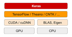
We will use the Keras library for our code sample. It turns out that the author of the book we referenced earlier (François Chollet) is also the author of this library. I really like this library because it sits on top of deep learning libraries like Tensor Flow and CNTK. Not only does it hide the complexity of the underlying framework, but it also provides a first-class notion of a neural network layer as a building block that all of us developers can appreciate. As you will see in the code example below, putting together a neural network becomes a simple matter of stacking these building blocks.

Let us review an elided version of a Python program that matches the neural network we discussed above. I don’t expect you to pick up every syntactic detail associated with the entire program. My goal is to map, at a high level, the concepts we talked about, to code. For a complete listing of code see this link. You can easily execute this code by provisioning an Azure Data Science Virtual Machine (DSVM) that comes preconfigured with an AI and data science development environment. You also have the option of provisioning the DSVM with GPU support.

// Import Keras

// Load the MNIST database training images and labels (fortunately it comes built into Keras)

// Create a neural network model and add two dense layers


// Define the optimizer, loss function and the metric

// It is not safe to feed the neural network large value (in our case integers
// ranging from 0-255. Let us transform it into a floating-point number between 0-1


// Start the training (i.e. fit our neural network into the training data)

// Now that our network is trained, let us evaluate it using the test data set


// Print the testing accuracy

// 97.86% Not bad for our very basic neural network

Not to denigrate what we have learned so far, but please keep in mind that the neural network architecture we have discussed above is far from the state of art in neural networks. In future blog posts, we will get into some of the cutting-edge advancements in neural networks. But don’t be disheartened, the neural net we have discussed so far is quite powerful with an accuracy of 97.86%.

Learn More About Neural Networks (But Don’t Anthropomorphize)

I don’t know about you, but it is pretty amazing to me that a few lines of code have given us the ability to recognize sloppily handwritten digits that our program has not seen before. Try writing such a program using the traditional programming techniques you know and love. Note however that our trained neural network does not have any understanding of what the digits mean (for example, our trained neural network will not be able to draw a digit, despite having been trained on 60,000 handwritten images)

I also don’t want to minimize the challenges involved in effectively using neural networks, starting with putting together a large training set. Additionally, the data wrangling work involved in transforming the input data into a format that is suitable for training the neural network is quite significant. Finally, developing an understanding of the various optimization techniques for improving the accuracy of our training can only come through experience (Fortunately, AutoML techniques are making the optimization much easier).

Hopefully, this blog post motivates you to learn more about neural networks as a programming construct. In future blog posts, we will look at techniques to improve the accuracy of neural networks, as well as review state of the art neural network architectures.